A 12-year study of the Q1 → Q2 → Q3 chain on NQ and ES. What lifts the marginal, what’s just baseline range expansion, and where the structural edge actually lives.
The Quarter framework
The 24-hour Globex session in equity index futures starts at 18:00 New York time and runs to the next 18:00. We split it into four 6-hour blocks measured from that anchor. The blocks are not labeled by session for a reason — the time-block boundaries don’t align perfectly with cash-market open/close hours (Tokyo, London, NY cash each start at hours inside the blocks, not at the boundaries). For this study, the blocks are pure time windows: Q1 is the first 6 hours after the Globex open, Q2 the next 6, and so on.
The four quarters per trade day:
| Quarter | Window (NY time) | Length |
|---|---|---|
| Q1 | 18:00 → 00:00 | 6 hours |
| Q2 | 00:00 → 06:00 | 6 hours |
| Q3 | 06:00 → 12:00 | 6 hours |
| Q4 | 12:00 → 18:00 | 6 hours |
The Q-Chain question is narrow and testable. If Q2 takes out a Q1 extreme — high or low — how often does Q3 extend the move past Q2’s extreme as well?
We call it a bull chain when Q2’s high breaks Q1’s high, and a bear chain when Q2’s low breaks Q1’s low. Continuation is binary: Q3’s high breaks Q2’s high (bull) or Q3’s low breaks Q2’s low (bear). The chain “fails” if Q2’s break stalls and Q3 never extends.
The framework itself is not new — variants of session-relay analysis (overnight → morning continuation) appear in multiple trading literatures. What this study contributes is twelve years of unfiltered intraday data, cohort-conditional probabilities with confidence intervals, and an honest accounting of what the chain condition actually adds on top of baseline range expansion.
Definitions and tie-breaks
Precision matters more here than in most studies because the chain framework involves a sequence of conditional events. We define every term explicitly:
- Trade day — the 24-hour window from 18:00 ET on calendar day N−1 to 18:00 ET on calendar day N. Labeled by the destination calendar date. So Sunday 18:00 ET starts the “Monday” trade day.
- Q1 / Q2 / Q3 / Q4 — four 6-hour quarters of the trade day in chronological order, as above.
- Qn high / low — maximum high / minimum low of all 1-minute bars whose timestamp falls inside the quarter’s window. Wick-inclusive.
- Chain formation — Q2 wick breaks Q1’s extreme. Bull chain: any bar in Q2 has high > Q1 high. Bear chain: any bar in Q2 has low < Q1 low.
- Both broken (tie-break) — if Q2 breaks both Q1’s high AND Q1’s low, the chain is assigned to the side with the larger excursion past Q1’s extreme (measured as fraction of Q1’s range).
- Continuation (chain success) — Q3 wick takes out Q2’s extreme in the same direction. Bull: any Q3 bar has high > Q2 high. Bear: any Q3 bar has low < Q2 low.
- Failure — Q3 ends at 12:00 ET without taking out Q2’s extreme.
- Chain-active day — any day where a chain formed (Q2 broke at least one Q1 extreme).
- Chain-inactive day — Q2 stayed strictly inside Q1’s range.
- Marginal rate — the plain success rate of a signal averaged over all qualifying days, with no further conditioning. “Bull chain marginal 77.6%” means 77.6% of all bull-chain days saw continuation.
- Null baseline — what you’d get by ignoring the chain entirely: the rate at which Q3 takes out Q2’s extreme on every day, chain or not. The honest yardstick for measuring whether the chain condition adds anything.
- Lift (percentage points, “pp”) — the gap between two rates, stated as a simple subtraction. A move from a 72% baseline to a 77% rate is a +5pp lift (not “+5%”). Percentage points avoid the ambiguity of percent-of-a-percent.
- Days — sample size. Throughout, every probability is followed by the number of historical trade days it was computed from; more days = more reliable.
All metrics use wick-based breaks (not closes). This is the natural convention for live decision making — a wick break is observable in real time, a close beyond a level only at the bar’s end.
Selection effect — how often the chain forms
Before any conditional probability is meaningful, the reader needs to know the denominator. The chain framework only applies on days where Q2 actually breaks Q1. On the rest, there’s no chain to discuss.
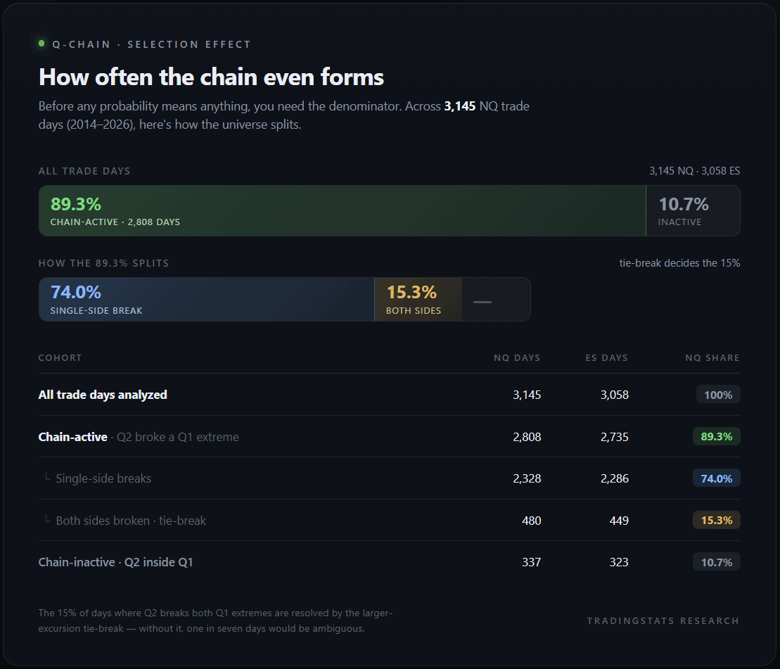
About 89% of trade days have a chain. The remaining 11% have a Q2 that respected Q1’s range entirely. These are typically low-volatility Q1+Q2 windows or pre-event compression days — they’re excluded from chain probabilities because the chain framework doesn’t apply.
The “both sides broken” cohort (15%) is the interesting one. On these days Q2 took out Q1 in both directions, so the tie-break rule kicks in and assigns the chain to the side with the larger excursion. Without this rule, ~15% of trade days would be ambiguous.
The honest baseline
Here is the marginal Q-Chain continuation rate on NQ and ES, computed across all chain-active days:
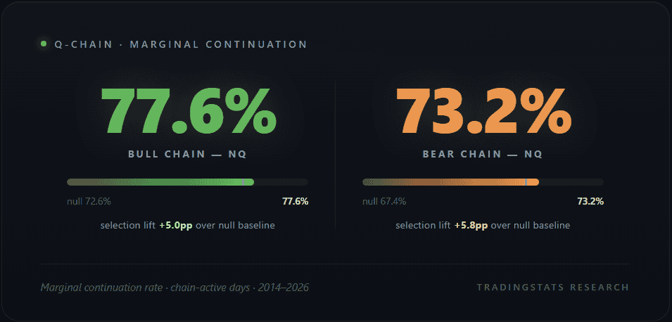
These numbers look strong. But they’re misleading without context.
The chain condition is itself a selection on directional price action: Q2 has already moved past Q1’s extreme. Some of the “continuation” rate is just baseline range expansion — Q3 is the busiest 6-hour window of the trade day on equity index futures, and on any normal day it tends to extend past the prior Q2 extreme regardless of whether a chain technically formed.
To quantify how much edge the chain condition actually adds, we compute the same continuation question on all trade days, not just chain-active ones. The null hypothesis: P(Q3 high > Q2 high) and P(Q3 low < Q2 low) on every day:
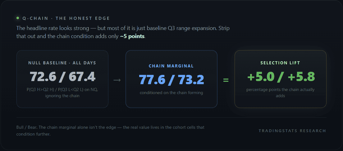
The chain condition adds roughly five percentage points of continuation rate on top of the baseline Q3 range-expansion tendency. Most of the headline “77.6%” is already there on a random day.
ES tells the same story. Null bull baseline is 69.3%, chain marginal is 75.0% — selection lift of +5.7pp. Null bear baseline is 62.2%, chain marginal is 66.9% — lift of +4.7pp.
This is the most important methodological point in the article. The chain marginal alone is not where the edge sits. Reading “bull chain → 77% to continue” as the whole story captures only ~5pp above what the same expectation would give on every single day, chain or not. That gap is small once real-world frictions are considered.
The real value of the Q-Chain framework is not the marginal — it’s the cohort conditioning that comes next.
Where the real edge lives — cohort cells
The marginal averages over all chain-active days. Within that pool, the days are very different from one another. A bull chain with a wide Q1, a small Q2 magnitude, and a chop-prone day of the week behaves nothing like a bull chain with a narrow Q1, a medium Q2 break, and Friday’s directional rhythm. Conditional probabilities split by cohort tell the real story.
We split chain-active days by:
- Q1 size — narrow / normal / wide, measured against the average Q1 range of the last 14 days (so “wide” means wide relative to recent volatility, not in absolute points)
- Q2 magnitude — tiny / small / medium / large, normalized by the day’s own Q1 range
- Day of week — Mon / Tue / Wed / Thu / Fri
This gives a 3 × 4 × 5 = 60-cell matrix per chain direction. Cells with fewer than 30 days of history are dropped (small-sample noise). The remaining cells span a wide spread — from about 65% (chop-prone cohorts) to over 90% (committed-directional cohorts).
A representative slice of high-probability cells on NQ, sorted by a conservative lower-bound estimate of the true rate (the Wilson method, which penalizes small samples so a 90% rate on 25 days ranks below a 85% rate on 200 days):
| Cohort (chain × Q1 size × Q2 mag × DOW) | P(continuation) | Lift vs null | Days |
|---|---|---|---|
| bull · normal · large · Thu | 92.1% | +19.5pp | 38 |
| bull · wide · tiny · Mon | 91.9% | +19.3pp | 37 |
| bull · wide · small · Fri | 85.7% | +13.1pp | 56 |
| bear · normal · large · Fri | 84.4% | +17.0pp | 32 |
| bull · wide · medium · Fri | 84.0% | +11.4pp | 50 |
| bull · wide · tiny · Fri | 82.6% | +10.0pp | 23 |
| bear · wide · medium · Fri | 82.0% | +14.6pp | 50 |
| bull · wide · large · Mon | 80.9% | +8.3pp | 68 |
The top cohorts deliver +10 to +19pp of lift over the null baseline — two to four times the lift of the chain marginal alone. This is where the framework’s structural edge lives.
What ties the high-probability cells together is committed directional context. They tend to be wide-Q1 days (lots of Q1+Q2 range to fade against), with small-to-medium Q2 breaks (Q2 broke decisively but didn’t overextend), on days of week with established directional bias (Friday close-out flow, Monday trend continuation).
The full cell matrix on NQ produces 46 published cells after applying two filters: at least 20 days of history per cell, and a conservative (Wilson lower-bound) continuation rate of 70% or better. The remaining cells either lack sample size or sit too close to the null baseline to be worth distinguishing from noise.
The P12 filter — side matters, regime doesn’t
The cohort cells condition on intraday structure (Q1, Q2, DOW). The P12 layer adds a Q1+Q2 shape conditioning: the combined Q1+Q2 range (call it P12, “period 12” in some literatures) has a midpoint, and where the directional close — Q2’s close — sits relative to that midpoint carries information.
Specifically: if a bull chain ends Q2 with Q2’s close above the P12 midpoint, the Q1+Q2 window ended directionally in agreement with the chain. If Q2’s close is below the P12 midpoint despite Q2 having broken Q1’s high, the chain is structurally weak — Q2 spiked above, then closed back down. The two cohorts are very different.
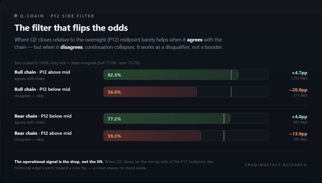
The agree cohorts add a modest +4.0 to +4.7pp on top of the marginal — a small structural confirmation. The disagree cohorts collapse the edge: bull chain with P12 closing below midpoint drops continuation rate by ~21 percentage points, from a 77.6% marginal down to 56.8% — barely better than a coin flip. The bear-side disagree drop is −13.9pp on NQ.
The P12 layer’s value is not as a confirmation booster — it’s as an anti-edge filter. Its main job is identifying days where the Q2 close contradicts the chain direction, and flagging them to skip.
The takeaway: the ~+4.5pp lift on agreement is real but minor on its own; the −21pp drop on disagreement is the meaningful finding. The P12 SIDE check works mainly as a disqualifier — when Q2 closes on the wrong side of the P12 midpoint relative to the chain direction, the historical continuation rate inverts sharply.
P12 regime — narrow / normal / wide
We also tested whether P12 regime (the size of the Q1+Q2 range, narrow / normal / wide vs rolling baseline) carries independent information. It mostly doesn’t:
| Chain × P12 regime cohort | P(continuation) | Lift vs marginal |
|---|---|---|
| Bull chain · P12 narrow | 80.2% | +2.7pp |
| Bull chain · P12 normal | 73.7% | −3.8pp |
| Bull chain · P12 wide | 78.1% | +0.7pp |
| Bear chain · P12 narrow | 73.7% | +1.5pp |
| Bear chain · P12 normal | 74.3% | +2.1pp |
| Bear chain · P12 wide | 68.1% | −4.1pp |
Lifts range from −4 to +3pp, all within the noise floor. The narrow regime on bull chains nudges up modestly, the wide regime on bears nudges down modestly, but neither magnitude is large enough to call a structural finding. P12 SIDE does the real work; P12 regime is informational at best.
Live time decay through Q3
The cohort cell gives the historical probability that the chain continues by Q3’s close. But during Q3 itself, that probability is dynamic — it depends on how much time has passed without continuation and where price currently sits relative to the target.
We pre-compute a decay table from the 12-year sample: at each 30-minute checkpoint between 06:00 and 11:30 ET, and for each of four distance buckets (how far price currently sits from the target, measured in multiples of a typical Q1 range: very close ≤0.25× / close ≤0.5× / far ≤1.0× / very far >1.0×), the conditional probability that the target is hit before 12:00 ET given the current state.
A representative slice of the bull decay table on NQ:
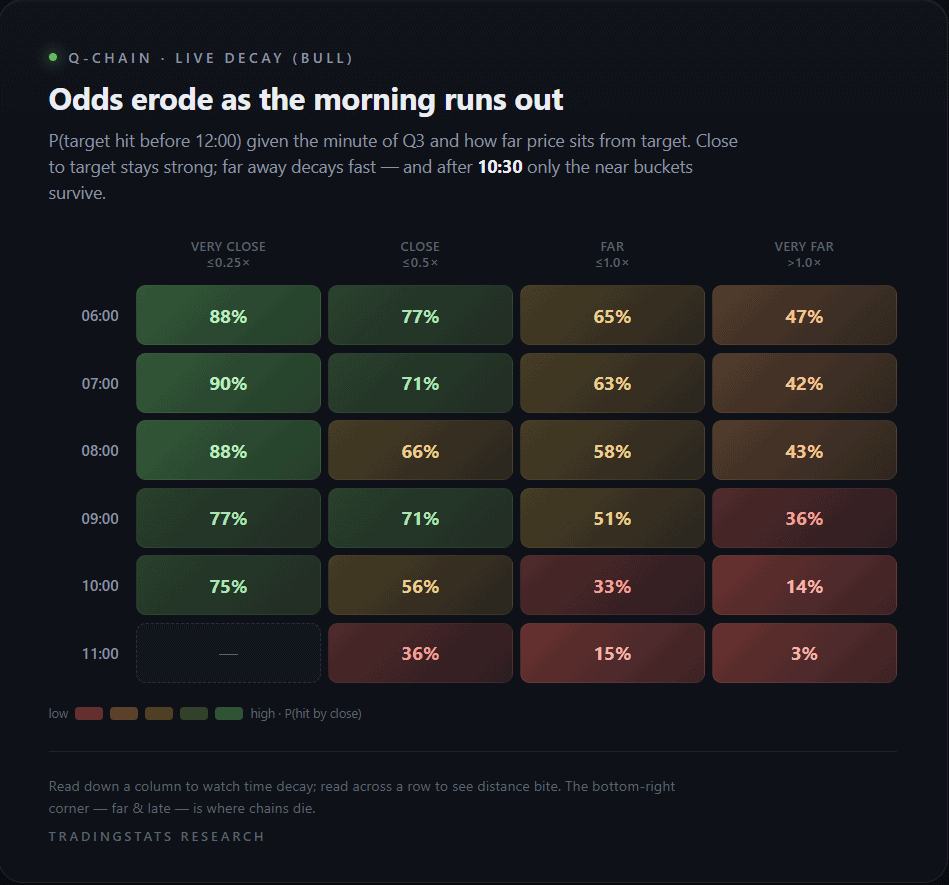
The pattern is intuitive. Close to target (VC bucket), probability stays high through most of Q3 — if price is hugging the target, it usually finishes the job. Far from target (VF bucket), probability degrades sharply as time runs out. After 10:30 ET, only the close-to-target buckets retain meaningful odds.
Read live during Q3, the decay table answers the question “given current price-to-target distance and current minute of Q3, what’s the residual probability the target gets hit before the close?” The answer can degrade sharply through the morning even on cohorts that had strong opening base rates.
Distance to target — the single strongest signal
Of every conditioning variable tested, one stands out for both strength and simplicity: how far price already sits from the target at the moment Q3 begins. The target is Q2’s extreme — the level Q3 must take out to continue. At 06:00 ET (Q3 open) we measure the gap from the current price to that target, normalized by the same 14-day Q1 range used elsewhere, and bucket it.
| Distance to target at 06:00 (× Q1 ATR) | Bull P(cont) | Bull days | Bear P(cont) | Bear days |
|---|---|---|---|---|
| Very close — < 0.10× | 93.1% | 248 | 96.4% | 84 |
| Close — 0.10–0.25× | 86.3% | 422 | 86.5% | 237 |
| Far — 0.25–0.50× | 77.5% | 448 | 77.9% | 375 |
| Very far — 0.50–1.0× | 64.8% | 338 | 62.7% | 378 |
| Extreme — ≥ 1.0× | 51.7% | 120 | 54.8% | 157 |
The spread is ~41 percentage points top to bottom — wider than any cohort cell, and almost perfectly monotonic on both chains. Distance to target is the strongest single predictor in the entire study.
The mechanism is not subtle, which is exactly why it’s trustworthy: if Q2’s extreme is already within 10% of a typical Q1 range of the current price, Q3 only has to nudge a little further to continue — it does so 93–96% of the time. If the target sits a full Q1 range or more away, Q3 has to manufacture a large directional move from scratch in six hours, and continuation falls to a coin flip (52–55%).
Unlike the cohort cells — which are fixed the moment the chain classifies at 06:00 — this measure updates with price: it answers “how reachable is the target from here?” with a clean, large-sample number. Combined with the time decay above, it forms the live core of the framework: distance sets the opening odds, decay erodes them as the morning runs out.
Anchor robustness
The whole framework rests on anchoring the trade day at 18:00 ET (CME Globex daily open). This is a defensible choice — it matches the actual session reset — but it’s also a parameter, and parameters need stress-testing. We recomputed the chain marginals under three different trade-day anchors:
| Anchor (NY time) | Chain-active % | NQ bull continuation | NQ bear continuation | Δ vs 18:00 |
|---|---|---|---|---|
| 18:00 (Globex open, canonical) | 89.3% | 77.6% | 73.2% | — |
| 16:00 (RTH close) | 88.7% | 73.2% | 70.1% | −4.4 / −3.1pp |
| 00:00 (calendar midnight) | 98.3% | 57.3% | 45.5% | −20.3 / −27.7pp |
The 18:00 ↔ 16:00 comparison is the meaningful test. Both are market-structure-aligned anchors (Globex open, RTH close) and both produce continuation rates within ~3–4pp of each other, with near-identical chain-active rates (~89%). The framework is robust to ±2 hours of session-aligned anchor choice.
The 00:00 calendar anchor collapses the framework — continuation drops 20–28pp. This is informative in the other direction: the chain edge is structurally tied to the market’s natural session rhythm. Splitting the trade day at calendar midnight slices through the middle of Q2, destroying the rhythm. The edge isn’t an arbitrary calendar artifact; it requires market-structure anchoring to exist at all.
Cross-instrument validation
We computed the same chain marginals on NQ, ES, YM and RTY:
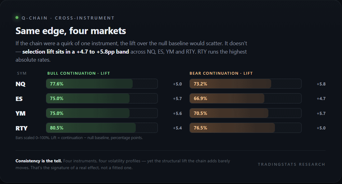
The four equity index futures behave nearly identically. Selection lift sits in a tight band across instruments (+4.7 to +5.8pp). RTY has the largest absolute continuation rates (highest baseline range expansion, characteristic of higher-volatility small-caps), but the structural lift the chain condition adds is consistent everywhere. This is the regime-independence proxy — if the framework were specific to one instrument’s quirks, the lift would differ markedly. It doesn’t.
DOW asymmetry — is there a “bear Monday” anti-edge?
Day-of-week is one of the cohort dimensions, so it’s worth asking whether any specific weekday changes the bear-chain odds. The short answer for Monday: not at the level that matters.
Marginal bear chain on Monday — 66.7% continuation (216 days on NQ, full 2014–2026 sample). That sits just below the other weekdays (bear Tue 73.9%, Wed 75.9%, Thu 71.0%, Fri 77.9%) — modestly the weakest bear day, but well within normal range and nowhere near an anti-edge.
For reference, the full bear-chain × DOW grid on NQ:
| Chain | Mon | Tue | Wed | Thu | Fri |
|---|---|---|---|---|---|
| Bull | 77.9% | 76.5% | 75.2% | 77.7% | 81.0% |
| Bear | 66.7% | 73.9% | 75.9% | 71.0% | 77.9% |
(Trade-day labeling is anchored at 18:00 ET, so Sunday-evening Globex correctly maps to the Monday trade day — verified against the raw bars. The DOW cells are not off by one.)
A note on small sub-cells. Slice bear × Monday further by Q1-size and Q2-magnitude and you can find a deep cell printing ~38.9% on just 18 days. That number is real in the data but is essentially noise: the 95% confidence interval runs roughly 20–60%, so it spans everything from a strong reversal pattern to a coin flip. It is not a tradeable anti-edge, and it should not be read as “Monday bear chains fail.” The marginal (66.7% over 216 days) is the honest figure.
The takeaway: there is a mild Monday softness on the bear side (~5–7pp below the strongest days), consistent with weekend-positioning unwinds occasionally reversing early Q3 selling. But it is a small marginal effect, not the dramatic flip a single low-n sub-cell might suggest. Any DOW-specific trading rule needs a longer or cross-instrument-pooled sample before it earns conviction.
Key takeaways
- The Q-Chain framework’s structural edge is real, but smaller than the marginal suggests. Chain forms on ~89% of trade days. Marginal continuation is 77.6% bull / 73.2% bear on NQ. Selection lift over the null baseline is only +5–6pp.
- The actual edge lives in cohort cells. Top conditioned cells (chain × Q1 size × Q2 mag × DOW) deliver +10 to +19pp lift over the null. Two to four times the lift of the chain marginal alone.
- P12 SIDE is the filter that matters. Disagreement between chain direction and P12’s directional close erodes continuation rate by 14–21pp — strong anti-edge.
- P12 REGIME doesn’t matter. Narrow / normal / wide P12 size adds only ±0–4pp of lift — informational, not actionable.
- Distance to target is the strongest single signal. Measured at Q3 open, continuation runs 93–96% when the target is within 0.10× a typical Q1 range, falling to 52–55% when it sits a full range or more away — a ~41pp spread, wider than any cohort cell and almost perfectly monotonic.
- Time decay is steep after 10:30 ET. Live probability drops sharply once the morning expands range; by 11:00 ET, only close-to-target buckets retain meaningful odds.
- 18:00 anchor is robust. Within ±2 hours of session-aligned alternatives the framework holds (~3–4pp). Calendar-midnight anchor collapses the edge entirely (−20 to −28pp), confirming the edge is market-structure-bound, not arbitrary.
- Cross-instrument consistency holds. NQ, ES, YM, RTY all show +4.7 to +5.8pp selection lift. RTY carries the highest absolute continuation rates (80.5/76.5). The framework is not instrument-specific.
- No real “bear Monday” anti-edge. Marginal bear-chain Monday continuation is 66.7% (216 days) — mildly the weakest bear weekday but normal. The dramatic 38.9% figure is a single deep sub-cell (18 days) and is statistical noise, not a tradeable signal.
From research to live tool
Every number in this study — the cohort cells, the P12 SIDE filter, the distance-to-target buckets, the intraday decay curves — is being wired directly into the TradingStats web app. Instead of reading a static table and mentally mapping it onto a live chart, you get the relevant probability computed automatically for the session in front of you.
In practice that means: the moment a chain forms at 06:00 ET, the platform classifies the day’s cohort (Q1 size, Q2 magnitude, day of week), reads the current distance to target, and surfaces a single live continuation probability — then decays it through Q3 as time passes and price moves. The P12 SIDE check fires its anti-edge warning automatically when the Q2 close contradicts the chain. No manual lookup, no spreadsheet, no guessing which cell applies.
The goal is to compress all of the above into instant context: open the chart, see whether today’s session sits in a high-base-rate cohort or a near-coin-flip one, and how much of the historical move is already accounted for by the clock. The research is the foundation; the app turns it into a real-time read so you spend your time on analysis, not arithmetic.

FAQ
Why use wick breaks, not closes, to define chain formation?
Wick breaks are observable in real time — the moment a 1-minute bar prints high > Q1 high, the chain has formed. Close-based definitions delay the signal by up to 30 minutes (if a 30M close were required) and would shrink the chain-active sample meaningfully. Wick-based is the standard convention for any live-trading framework built on level breaks.
Why 18:00 ET specifically, and not other reasonable anchors?
18:00 ET is the CME Globex daily reset — the moment all equity index futures roll their session counters. It’s the most structurally significant anchor available. We tested 16:00 (RTH close) and 00:00 (calendar midnight) as alternatives: 16:00 produces nearly equivalent results, 00:00 destroys the edge. The framework is robust to any anchor within the trading day’s natural rhythm.
Can the 85–92% top cells be used directly?
This study is descriptive, not advice. The top cells have lifts of +10 to +19pp over the null baseline, which is meaningfully better than the marginal — but cell sample sizes are 30–70 days, the confidence intervals are wide (±10–15 percentage points), and the cohort filter is computed from 12 years of data with no out-of-sample reserve. Treat the findings as hypotheses to study further, not as instructions.
Why does the P12 regime filter add so little?
Likely because P12 size (the range of Q1+Q2 combined) is highly correlated with the day’s expected volatility, which in turn correlates with Q3’s range. Conditioning on P12 size mostly conditions on something already baked into the cell’s Q1 size dimension. The P12 SIDE, by contrast, captures directional commitment that Q1 size doesn’t — which is why it adds independent information.
Does the framework hold on non-equity instruments?
We haven’t tested it on bonds, energy, or metals. The Q1 → Q2 → Q3 rhythm is calibrated to equity index intraday liquidity flow. Other asset classes have different intraday volume profiles — gold’s most active hours, for example, sit differently within the 24-hour window. A separate study is warranted.
Is there look-ahead bias in the cohort assignments?
No. Q1 size is normalized by a 14-day rolling Q1 range, shifted by one day so today’s classification uses only prior sessions. Q2 magnitude is normalized by the day’s own Q1 range, which is fully known by 06:00 ET when the chain classification fires. All cell lookups happen at or after the Q3 start.
The chain marginal lift is only +5pp — is the framework worth using at all?
The marginal is the wrong number to focus on. The framework’s value sits in the cohort-conditional rates (the Q1-size × Q2-magnitude × DOW cells), the P12 SIDE filter that flags when the Q2 close contradicts the chain, and the time decay through Q3. Those collectively deliver +10–19pp lift in favorable cohorts and flag explicitly when the cohort degrades. The marginal is a starting point; the cohort layer is where the structural edge lives.