Standard Deviation Trading: What 12 Years of Futures Data Actually Show

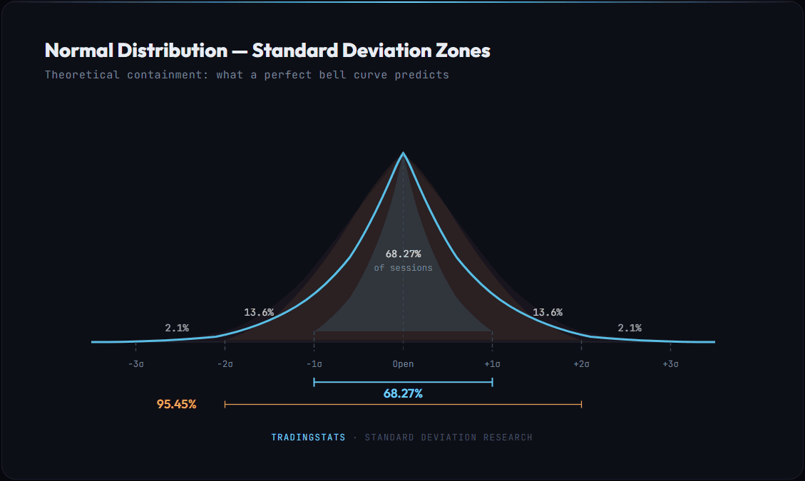
Every options pricing model, every risk manager, and every volatility indicator is built on the same premise: price tends to stay within a statistically defined range. The standard deviation of returns defines that range. At 1 standard deviation, the normal distribution says 68.27% of observations should fall inside. At 2 standard deviations, 95.45%. At 3 standard deviations, 99.73%.

But futures markets are not normal distributions. We tested this directly — not with theory, not with textbook examples, but with 12 years of 1-minute bar data across four US equity index futures: NQ (Nasdaq 100), ES (S&P 500), YM (Dow Jones), and RTY (Russell 2000).

This article presents what we found: actual containment rates, hit rates, reversal probabilities, fat tails, and where the normal distribution breaks down. No trading signals. No setups. Just measured statistics from over 3,000 trading days.

What Is Standard Deviation in Trading?

Standard deviation (SD) measures how much returns typically deviate from the average. In futures trading, this is applied to price movements from a reference point — usually the session open. Many charting platforms offer a standard deviation indicator that plots these levels directly on price charts — similar to Bollinger Bands, but measured from the session open rather than a moving average.

If NQ has a daily SD of 1.06%, and today’s open is 20,000, then:

• +1 SD = 20,212 (the upper boundary of the “normal” daily range)
• -1 SD = 19,788 (the lower boundary)

The expectation, under a normal distribution, is that price will close within this range on roughly 68% of trading days.

The Rule of 16

There is a well-known shortcut for converting annualized volatility to daily volatility: divide by 16 (the approximate square root of 252 trading days). If the VIX reads 16, the market is pricing a 1% daily expected move for the S&P 500. If VIX is 24, the expected daily range is 1.5%.

This conversion works in reverse too. If a futures contract has a measured daily SD of 1.06%, the annualized volatility is roughly 1.06% × 16 = 17%.

Standard Deviation Trading Levels: Three Timeframes, Four Instruments

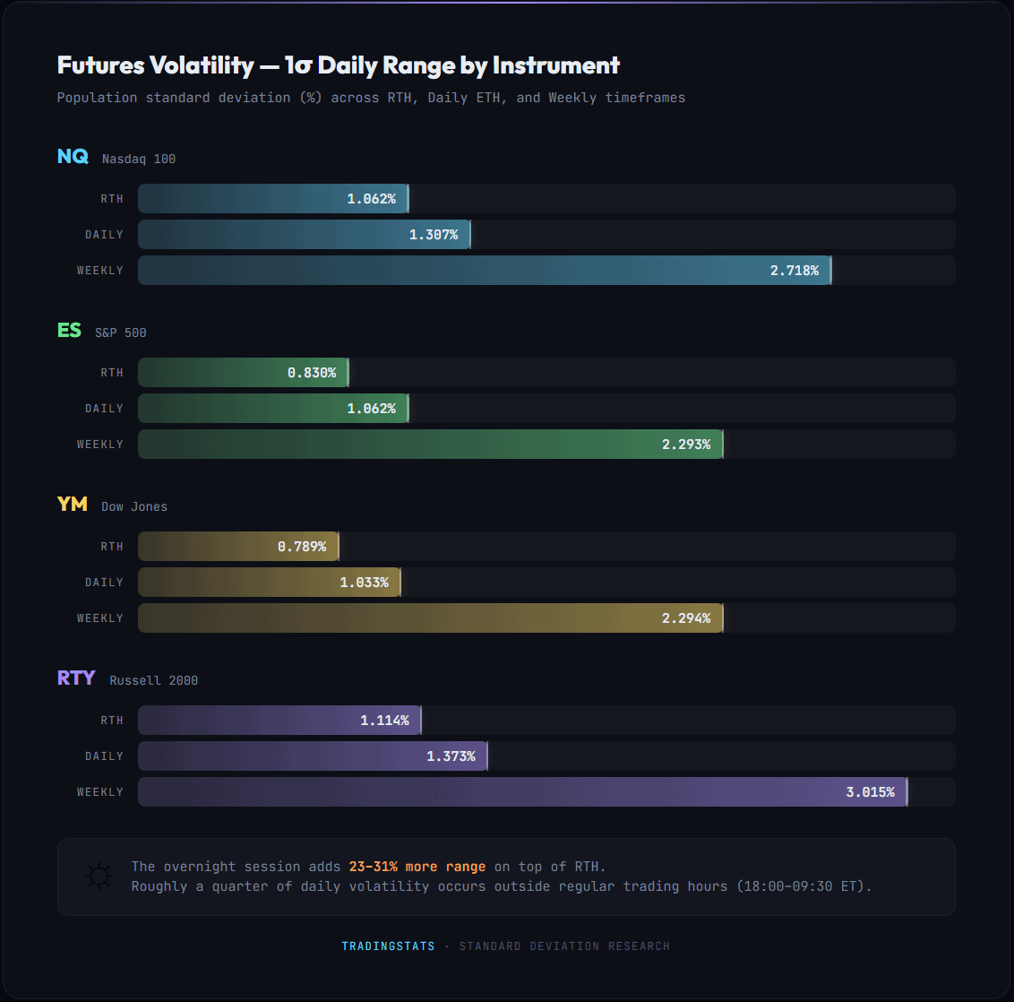
We calculated population standard deviation (STDEV.P) of open-to-close returns across three timeframes:

RTH (Regular Trading Hours: 09:30 – 16:00 ET)

This is the main session — the 6.5 hours when the NYSE and NASDAQ are open. SD is calculated from the RTH open price.

Instrument	1 SD (%)	At 20,000	At 5,000
NQ (Nasdaq 100)	1.062%	±212 pts	—
ES (S&P 500)	0.830%	—	±42 pts
YM (Dow Jones)	0.789%	—	±39 pts
RTY (Russell 2000)	1.114%	—	±56 pts

RTY is the most volatile instrument in percentage terms. NQ is close behind. YM is the quietest. These values define the expected daily range for each instrument — the boundaries within which price is statistically likely to close.

ETH Daily (18:00 ET – 17:00 ET next day)

The full 23-hour futures session, starting from the Globex open at 18:00 ET. This captures the overnight session, the European open, and the full US trading day. SD is calculated from the ETH open price.

Instrument	1 SD (%)	vs RTH
NQ	1.307%	+23% wider
ES	1.062%	+28% wider
YM	1.033%	+31% wider
RTY	1.373%	+23% wider

The full session adds roughly 23–31% more volatility compared to RTH alone. The overnight session is not “dead time” — significant price discovery happens between 18:00 and 09:30.

Weekly (Sunday 18:00 ET – Friday 17:00 ET)

Full trading week, from the Globex open on Sunday evening to Friday’s close. SD is calculated from the weekly open price.

Instrument	1 SD (%)	vs Daily ETH
NQ	2.718%	2.08x daily
ES	2.293%	2.16x daily
YM	2.294%	2.22x daily
RTY	3.015%	2.20x daily

Weekly SD is approximately 2x the daily SD — consistent with the square root of time rule (sqrt(5 trading days) = 2.24). RTY’s weekly SD of 3.015% means a typical weekly range of ±600 points from the open on a 20,000 price.

Is 1 Standard Deviation Always 68%? Theory vs. Reality

The most fundamental question: does price actually stay within 1 SD on 68% of days?

What the Normal Distribution Predicts

Range	Containment
Within ±0.5 SD	38.29%
Within ±1.0 SD	68.27%
Within ±1.5 SD	86.64%
Within ±2.0 SD	95.45%
Within ±3.0 SD	99.73%

What We Measured (RTH Sessions, 2014–2026)

SD Level	Theory	NQ (3,119 days)	ES (3,044 days)	YM (3,119 days)	RTY (3,119 days)
±0.5 SD	38.29%	50.98%	54.24%	53.77%	46.52%
±1.0 SD	68.27%	76.88%	78.71%	79.26%	74.96%
±1.5 SD	86.64%	89.36%	90.05%	90.86%	89.55%
±2.0 SD	95.45%	94.58%	94.71%	95.16%	95.00%
±3.0 SD	99.73%	98.40%	98.36%	98.46%	98.85%

The pattern is consistent across all four instruments: at 1 SD, the actual containment rate is 75–79% — 7 to 11 percentage points higher than the theoretical 68.27%. This is not a coincidence. It is a direct consequence of how financial returns are actually distributed.

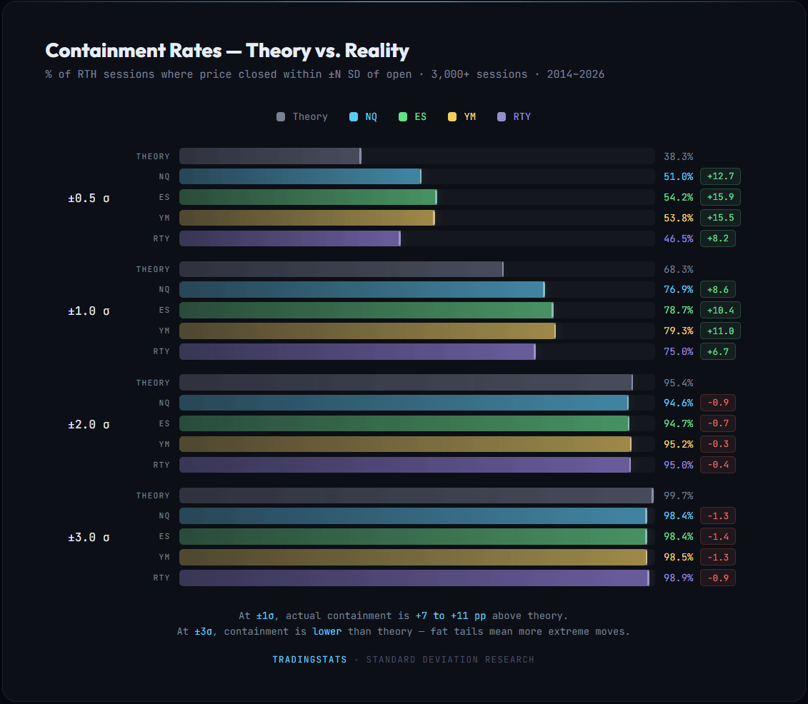
At 0.5 SD, the effect is even more pronounced: 47–54% containment versus 38% theoretical. Price clusters near the open more than a bell curve predicts.

But at 2 SD and beyond, the relationship flips. Observed containment at 3 SD is 98.4–98.9%, compared to the theoretical 99.73%. That gap — roughly 1 percentage point — may seem small, but it means extreme moves happen 4–6x more frequently than a normal distribution predicts.

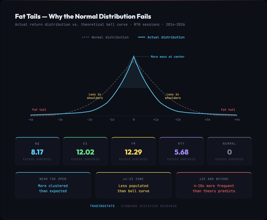
Fat Tails: Why the Normal Distribution Fails

Financial returns are not normally distributed. This has been documented extensively since Benoit Mandelbrot’s 1963 paper on commodity price variations and confirmed across every asset class studied since.

Kurtosis: The Shape of the Distribution

Kurtosis measures how “peaked” or “fat-tailed” a distribution is relative to a normal distribution. A normal distribution has excess kurtosis of 0.

Our measured excess kurtosis values for RTH daily returns: NQ = 8.17, ES = 12.02, YM = 12.29, RTY = 5.68. All are well above zero, meaning extreme events occur far more frequently than a bell curve predicts. The Jarque-Bera normality test rejects the normal distribution for all four instruments (p = 0.0). The distribution has:

• More mass near the center — price stays near the open more often than expected
• Less mass in the “shoulders” — the 1–2 SD zone is less populated
• More mass in the extreme tails — 3+ SD moves happen far more often

This creates a paradox: on most days, SD levels work better than theory suggests (higher containment). But on the days they fail, they fail spectacularly.

How Often Do Extreme Moves Happen?

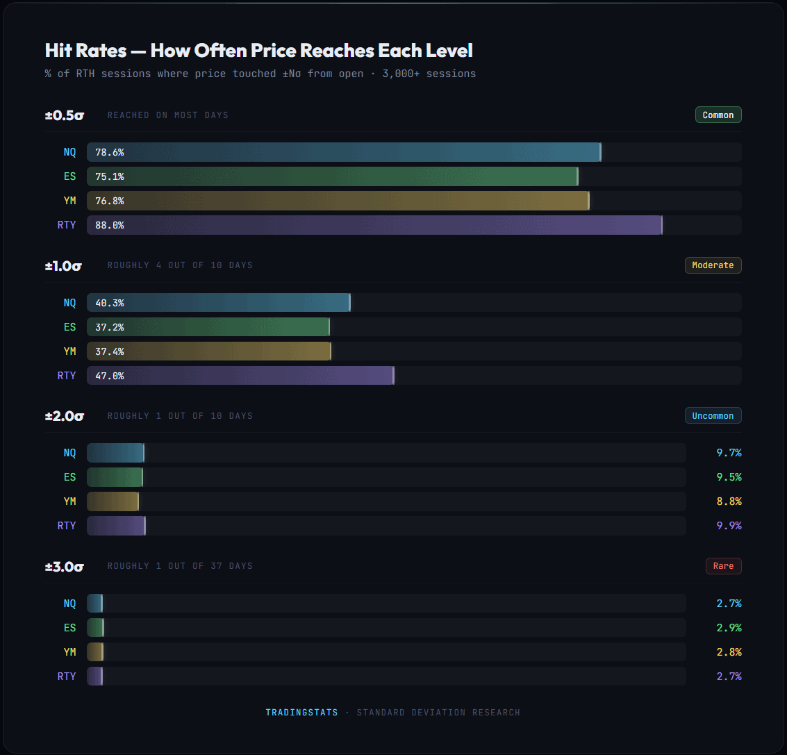
During the RTH session, price reaches each SD level (intraday high or low touches ±N SD from the open) on the following percentage of trading days:

SD Level	NQ	ES	YM	RTY	Normal (close-based)
±0.5 SD reached	78.6%	75.1%	76.8%	88.0%	61.7%
±1.0 SD reached	40.3%	37.2%	37.4%	47.0%	31.7%
±1.5 SD reached	19.8%	17.7%	17.7%	20.9%	13.4%
±2.0 SD reached	9.7%	9.5%	8.8%	9.9%	4.6%
±3.0 SD reached	2.7%	2.9%	2.8%	2.7%	0.27%

At 3 SD, the observed hit rate is roughly 10x the normal prediction. At 2 SD, it is about 2x. The discrepancy grows exponentially at the extremes.

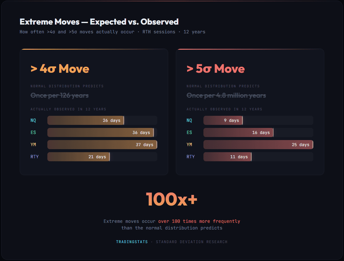
Over 3,000+ trading days, the number of days with extreme moves:

Move	NQ	ES	YM	RTY
> 4 SD	26 days (0.83%)	36 days (1.18%)	37 days (1.19%)	21 days (0.67%)
> 5 SD	9 days (0.29%)	16 days (0.53%)	25 days (0.80%)	11 days (0.35%)

A 4 SD daily move — also known as a 4-sigma event — “should” happen once in 126 years under a normal model. In our 12-year dataset, it happened 21–37 times depending on the instrument. A 5-sigma move should be virtually impossible — we observed 9–25 instances per instrument.

Distribution Shape: Kurtosis and Skewness

Instrument	Excess Kurtosis	Skewness	Days	Normal Rejected?
NQ	8.17	+0.08	3,119	Yes (p = 0.0)
ES	12.02	+0.18	3,044	Yes (p = 0.0)
YM	12.29	+0.12	3,119	Yes (p = 0.0)
RTY	5.68	−0.15	3,119	Yes (p = 0.0)

ES and YM show the highest kurtosis (12+), meaning the most extreme fat tails relative to a normal distribution. RTY has the lowest kurtosis (5.68) but the highest overall volatility. NQ sits in the middle at 8.17. All four show near-zero skewness — the distributions are roughly symmetric around the mean, but with dramatically heavier tails than a bell curve.

Hit Rates: How Often Does Price Reach Each Level?

A “hit” means that during the session, price reached at least ±N standard deviations from the open (either the high went above +N SD or the low went below −N SD).

RTH hit rates — percentage of trading days where price reached at least ±N SD from the open at any point during the session:

SD Level	NQ	ES	YM	RTY
±0.5 SD	78.6%	75.1%	76.8%	88.0%
±1.0 SD	40.3%	37.2%	37.4%	47.0%
±1.5 SD	19.8%	17.7%	17.7%	20.9%
±2.0 SD	9.7%	9.5%	8.8%	9.9%
±3.0 SD	2.7%	2.9%	2.8%	2.7%

The ±0.5 SD level is reached on the vast majority of trading days (75–88%). The ±1 SD level is reached approximately 37–47% of the time. The ±2 SD level is a relatively rare event, occurring on roughly 9–10% of days.

RTY stands out: it hits 0.5 SD on 88% of days and 1 SD on 47% of days — significantly more than the other three. This reflects RTY’s higher baseline volatility and lower kurtosis — moves are more spread out rather than clustered at the extremes.

This creates an asymmetry that matters: 1 SD is reached on 37–47% of all days, but price closes within 1 SD on 75–79% of days. That gap — between “touched” and “closed beyond” — is the reversal rate.

Reversal Rates: Touch Does Not Mean Continuation

This is perhaps the most practically relevant metric. When price reaches a given SD level during the session, how often does it close back inside that level?

Reversal rate = when price reaches ±N SD during the session, the percentage of times it closes back inside that level:

SD Level	NQ	ES	YM	RTY
±0.5 SD	37.6%	39.1%	39.8%	39.2%
±1.0 SD	42.6%	42.8%	44.5%	46.7%
±1.5 SD	46.1%	43.7%	48.3%	50.0%
±2.0 SD	43.9%	44.3%	44.7%	49.4%
±3.0 SD	41.2%	43.8%	44.8%	56.6%

The reversal rates are remarkably uniform across SD levels and instruments — mostly in the 38–50% range. This means that when price reaches any given SD level, it closes back inside that level less than half the time.

At ±1 SD, the reversal rate across all four instruments is 42–47% — not far from a coin flip, and below 50%. When price reaches 1 SD, it is more likely to close beyond that level than to reverse.

RTY shows the highest reversal rates, especially at 3 SD (56.6%) — consistent with its lower kurtosis. Its extreme moves are less likely to persist than those of NQ, ES, or YM.

Important nuance: A reversal rate below 50% does NOT mean the level is a reliable continuation signal. It means the levels are not reliable reversal points. The practical takeaway is that SD levels are reference points for measuring extremity, not inflection points for entries. Those looking for a standard deviation trading strategy with fixed entry rules will find that the data does not support one — the edge is in context, not in mechanical signals.

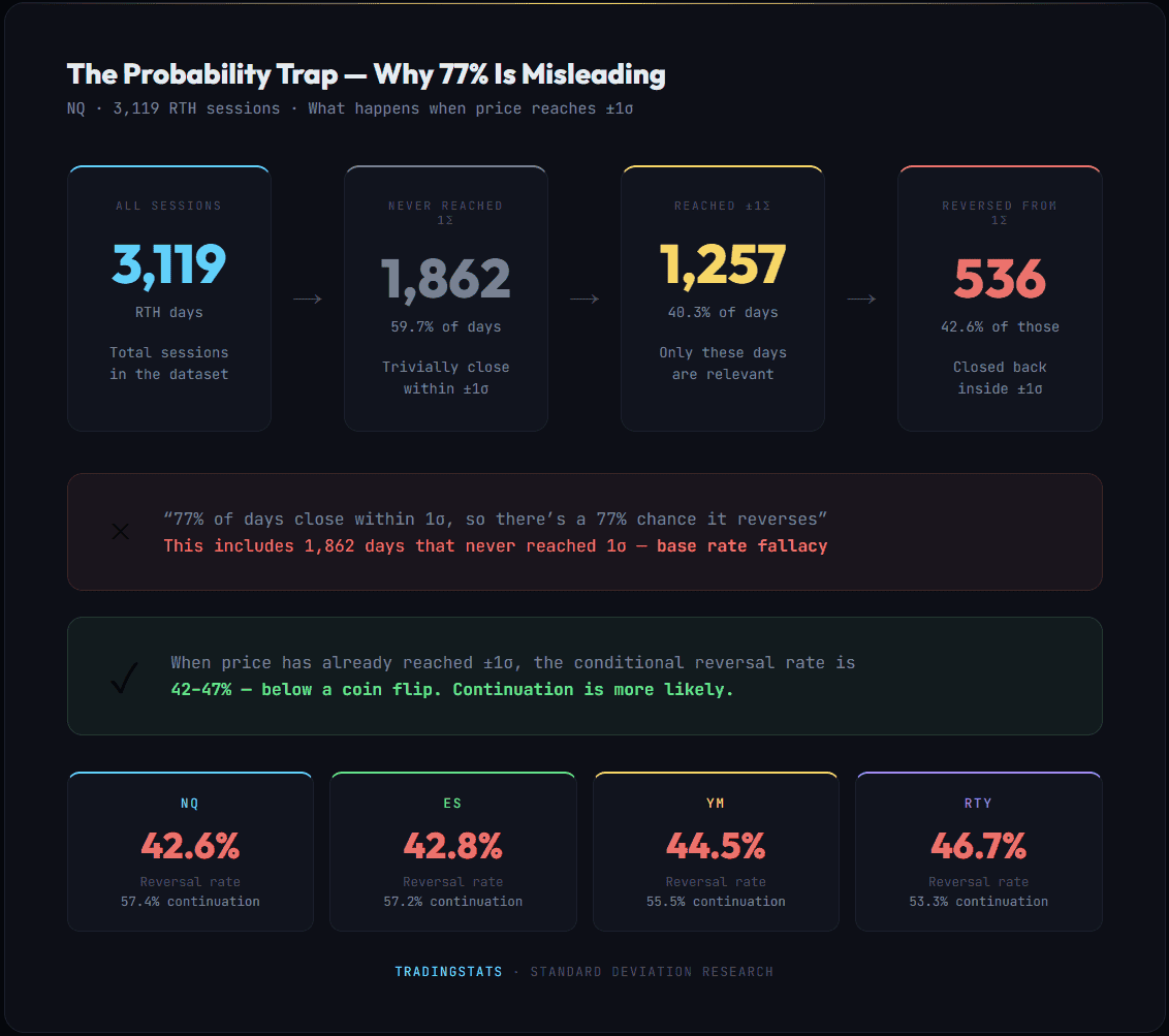
The Probability Trap: Why 77% Does Not Mean What You Think

Many traders use standard deviation levels as probability-based reversal zones. The logic sounds compelling: “If 77% of days close within 1 SD, then when price reaches 1 SD, there is a 77% chance it will come back.” This reasoning is wrong — and it is one of the most common misapplications of statistics in trading.

The Error: Unconditional vs. Conditional Probability

The 77% containment rate is an unconditional probability — it applies to a random day before the session starts. It includes all days, most of which never reach 1 SD at all:

For NQ (3,119 RTH days):

• Price never reached 1 SD: 1,862 days (59.7%) — all trivially close within 1 SD
• Price reached 1 SD: 1,257 days (40.3%) — the only days relevant to the question

Total containment: (1,862 + 536) / 3,119 = 76.9%. But 1,862 of those days have nothing to do with what happens when price is already at 1 SD.

The Correct Number: Conditional Reversal Rate

When price has already reached ±1 SD, the relevant statistic is the conditional reversal rate:

Instrument	Reversal at 1 SD	What it means
NQ	42.6%	57.4% of the time, price closes beyond 1 SD
ES	42.8%	57.2% continuation
YM	44.5%	55.5% continuation
RTY	46.7%	53.3% continuation

All below 50%. When price reaches 1 SD, the most likely outcome is that it stays beyond that level — not that it reverts.

Why NORM.DIST Gives Wrong Probabilities

Some trading tools and indicators calculate SD-level probabilities using Excel’s NORM.DIST function or its equivalent — applying the normal (Gaussian) distribution formula. This produces clean, mathematically precise numbers that are wrong.

NORM.DIST assumes a bell curve. Financial returns are not a bell curve. Our measured kurtosis (5.7–12.3) proves this. The consequences:

What NORM.DIST says	What the data shows	Error
68.3% close within 1 SD	75–79% close within 1 SD	Underestimates by 7–11 pp
95.4% close within 2 SD	94.6–95.2% close within 2 SD	Close, slightly overestimates
99.7% close within 3 SD	98.4–98.9% close within 3 SD	Overestimates (hides tail risk)
4 SD = once per 126 years	4 SD = 21–37 times in 12 years	Off by 100x+

At 1 SD, NORM.DIST makes you think containment is lower than it actually is. At 3+ SD, it makes you think extreme events are rarer than they actually are. Both errors can be costly.

The Correct Framework

Standard deviation levels are probabilistic — but the probability they represent is unconditional, not a prediction of what happens after price reaches the level. The distinction:

• Before the session opens: there is a ~77% probability that today’s close will be within ±1 SD of the open. This is useful for framing expectations.
• After price reaches 1 SD: the reversal probability drops to 42–47%. The 77% number no longer applies.

Using SD levels as “probability of reversal” is a base rate fallacy — applying a population statistic to a filtered subset where it does not hold.

Implied Volatility vs. Realized Volatility

There is a well-documented phenomenon in options markets: implied volatility (IV) systematically overestimates realized volatility. This is called the Variance Risk Premium.

Key findings from academic research:

• The VIX (S&P 500 implied volatility) overestimates subsequent 30-day realized volatility approximately 85% of the time
• The average overestimation is roughly 3–4 volatility points (e.g., VIX at 20, realized vol at 16)
• The premium is largest during calm markets and can briefly invert during sudden crashes

This has a direct implication for SD-based levels: if you derive them from implied volatility (as options expected moves do), price will stay within the boundaries more often than 68%. If you derive them from historical realized volatility (as we do), the containment rates are closer to, but still above, the theoretical values.

Daily Volatility Comparison: NQ vs ES vs YM vs RTY

Not all futures are created equal. Understanding futures volatility requires looking at actual measured data, not assumptions. The four major US equity index futures have meaningfully different volatility profiles:

RTY: The Most Volatile

Russell 2000 futures consistently show the highest SD across all timeframes. RTY’s daily RTH SD of 1.114% is 42% wider than YM’s 0.789%. Small-cap stocks are more volatile than large-caps — this is a well-established market structure phenomenon.

NQ: High Absolute Volatility, Driven by Tech

Nasdaq 100 futures have the second-highest percentage SD (1.062% RTH) but, given their high nominal price, produce the largest point moves. A 1 SD day on NQ at 20,000 is ±212 points — nearly $4,240 per contract.

ES: The Benchmark

S&P 500 futures sit in the middle of the volatility spectrum at 0.830% RTH. As the most liquid equity index future, ES has the tightest bid-ask spreads and the most predictable volatility behavior.

YM: The Quietest

Dow Jones futures have the lowest SD at 0.789% RTH. The Dow’s price-weighted methodology and concentration in mature industrials produces the narrowest daily ranges in percentage terms.

Overnight Adds ~25% More Range

Across all four instruments, the ETH daily SD is 23–31% wider than the RTH SD. This means roughly a quarter of total daily volatility occurs outside of regular trading hours. For traders who only watch the 09:30–16:00 session, significant price discovery is happening before they see it.

The Square Root of Time Rule

There is a mathematical relationship between volatility and time: volatility scales with the square root of time. If daily SD is X%, then weekly SD should be approximately X% × sqrt(5) = X% × 2.24.

Our measured values:

Instrument	Daily ETH SD	Weekly SD	Ratio	Theoretical (sqrt 5)
NQ	1.307%	2.718%	2.08x	2.24x
ES	1.062%	2.293%	2.16x	2.24x
YM	1.033%	2.294%	2.22x	2.24x
RTY	1.373%	3.015%	2.20x	2.24x

The measured ratios (2.08–2.22x) are consistently below the theoretical 2.24x. This makes sense: weekly returns include weekend gaps and week-long mean reversion that slightly compress the range compared to pure random walk scaling.

Standard Deviation as a Trading Indicator: What It Is (and What It Is Not)

Based on 12 years of data across four instruments, standard deviation levels are:

What they are:

• Statistically grounded reference points for daily, weekly, and session-level price ranges, commonly used in risk management to contextualize position sizing and exposure
• A measurement of historical volatility that tells you how far price typically moves
• More reliable than the normal distribution suggests — actual containment is higher than the textbook 68%
• A framework for understanding relative extremity: how stretched is today’s move compared to the historical norm

What they are not:

• Reversal signals — the reversal rate at ±1 SD is roughly a coin flip
• Precision levels — SD levels are round statistical boundaries, not support/resistance with order flow behind them
• Constant — volatility clusters and regime changes mean that today’s actual range may be significantly wider or narrower than the long-term average SD
• Normally distributed — fat tails mean the levels undercount extreme moves by orders of magnitude

The levels are most informative as a filter for extremity. When price is within ±0.5 SD of the open, nothing unusual is happening. When price reaches ±1.5 SD, the move is historically in the top 15–20% of sessions. When price reaches ±2 SD, you are in a statistically rare event — which may reverse, or may be the beginning of a fat-tail day that blows through every level on the chart.

Free TradingView Indicator: STDEV Levels

We built a free TradingView indicator that plots all the standard deviation levels from this research directly on your chart. The indicator uses the same empirical data presented above — 12 years of measured statistics, not theoretical values from NORM.DIST.

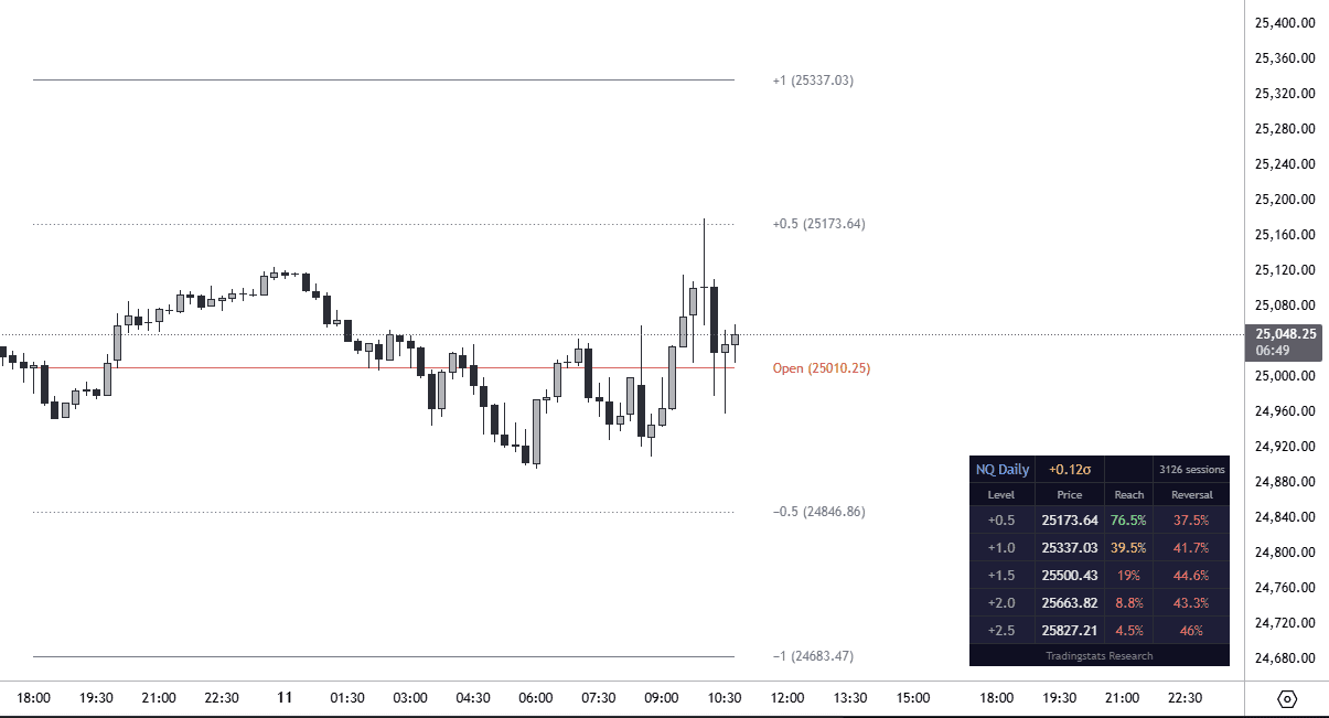
The indicator includes:

• Standard deviation levels at ±0.5σ, ±1σ, ±1.5σ, ±2σ, ±2.5σ, and ±3σ from session open
• Three timeframes: RTH, Daily (ETH), and Weekly — all can be displayed simultaneously
• A dynamic conditional probability table that updates in real time as price moves through levels
• Per-level customization: colors, line styles, and visibility toggles
• Support for NQ, ES, YM, RTY and their micro contract equivalents (MNQ, MES, MYM, M2K)

The probability table shows two key metrics for each level above the current price position: the conditional reach probability (how likely price is to reach the next level given it has already passed the current one) and the historical reversal rate.

Methodology

All statistics in this article are calculated from 1-minute bar data stored in Parquet format:

• Data source: Sierra Chart exports + InsightSentry API continuous contract data
• Period: 2014–2026 (~12 years, ~3,000+ trading days per instrument)
• Instruments: NQ (CME E-mini Nasdaq 100), ES (CME E-mini S&P 500), YM (CBOT E-mini Dow), RTY (CME E-mini Russell 2000)
• Standard deviation formula: Population standard deviation (STDEV.P / ddof=0) of open-to-close returns
• Timezone: All session boundaries in Eastern Time (America/New_York), including proper DST handling
• Session definitions:
  • RTH: 09:30–16:00 ET (NYSE/NASDAQ regular hours)
  • ETH: 18:00 ET – 17:00 ET next day (full Globex session)
  • Weekly: Sunday 18:00 ET – Friday 17:00 ET

No filtering for holidays, FOMC days, or earnings weeks has been applied. The statistics represent all available trading days.